1. Information about P&A Leakage Calculator
A PDF version can be downloaded here:
Consolidated web edition with legacy technical background
Application: OpenLab P&A Leakage Calculator
Prepared: April 2026
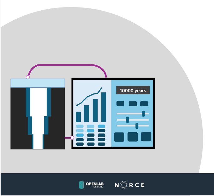
The OpenLab P&A Leakage Calculator is a web-based tool for evaluating leakage risk in permanently plugged and abandoned wells. It supports a risk-informed assessment of a proposed permanent well barrier system by estimating leakage through relevant barrier elements and failure mechanisms over a defined analysis period.
The calculator is intended to complement the prescriptive P&A design approach used in standards such as NORSOK D-010. Instead of only checking whether a barrier design satisfies a set of design rules, the calculator helps quantify how a given design may perform under uncertainty. The central questions are:
• What leakage rate may occur through the permanent barrier system?
• Which barrier, barrier element, or failure mode controls the result?
• How sensitive are the results to uncertain geometry, material, reservoir, and failure-mode assumptions?
• How does the result change with time as reservoir pressure and stress conditions evolve?
OpenLab provides a browser-based environment where users create configurations, start from templates, run simulations, and inspect results in an interactive result panel. The leakage models are based on NORCE research and computer models for leakage through plugged and abandoned wells.
The calculator can represent several leakage pathways:
• flow through bulk barrier material,
• flow through cracks,
• flow through microannuli along cement-casing interfaces,
• flow through microannuli along cement-formation interfaces,
• leakage through combinations of barrier elements and failure modes.
The tool should be treated as engineering decision support. It does not replace professional judgement, regulatory requirements, well-specific verification, or detailed project-specific risk assessments.
2. Account and login
The P&A Leakage Calculator is available at https://leakage.build.openlab.app/. Access is managed through the OpenLab login system.
2.1 Create an account
Open https://live.openlab.app/ in a web browser. If you do not already have an OpenLab account, you can request access using a Google or Microsoft account, as shown in the login window below.

Some functionality may depend on your account type, license, or project access. To unlock full functionality, run several simulations, or obtain access to additional OpenLab services, contact the OpenLab team or consult the OpenLab access and pricing information.
2.2 Browser recommendation
For the best user experience, Google Chrome is recommended. The application also runs in Microsoft Edge, Firefox, and Safari, although some interface components may appear differently. The calculator can be used on different screen sizes, including mobile devices, but some functions may be hidden or simplified on smaller screens.
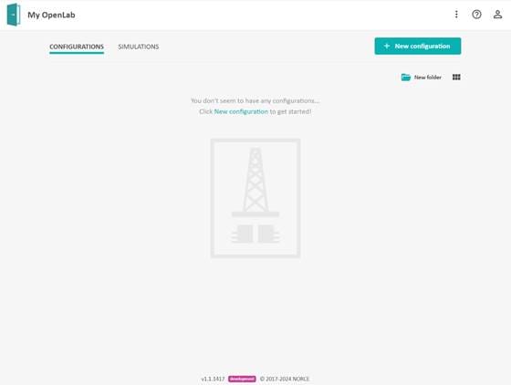
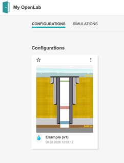
3. Home page and configurations
After login, OpenLab opens the Home page. This page gives an overview of your configurations and simulations.

From the Home page you can:
1. create new configurations,
2. open existing configurations,
3. copy, rename, move, or delete configurations,
4. access user-specific settings and account information,
5. return to the Home page by selecting the OpenLab icon in the upper-left corner.
3.1 What is a configuration?
A simulation in OpenLab is based on a configuration. A configuration describes the well, formations, reservoir conditions, barrier elements, material properties, uncertainty distributions, failure modes, and simulation settings used by the leakage models.
A configuration is not only a set of numerical inputs. It is the full description of the case to be simulated. It should therefore be named clearly and documented with sufficient assumptions and comments so that the case can be understood later by you or another user.
3.2 Templates
OpenLab provides template configurations to help users get started. A template can be copied and adapted to a specific well or study case. Use templates as starting points, not as validated engineering cases. The assumptions in the template should be checked before results are used.
3.3 Data management
Downloaded configurations are stored in a readable structured format, such as JSON in the web version. Treat these files as engineering data. They may contain well names, field names, geometry, assumptions, and other sensitive project information. Store and share them according to your organization’s data handling rules.
4. Configuration workflow
4.1 Create a configuration
A new well configuration can be created from the Home page. Select New configuration.
A dialog opens where the first configuration settings are defined.
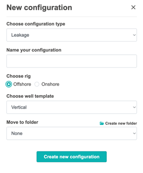
Fill in the required fields:
1. Configuration name - a descriptive name for the case.
2. Rig or well type - for example onshore or offshore.
3. Well template - the template used as the starting point for the configuration.
4. Folder - an existing or new folder where the configuration should be stored. This step can be skipped if the configuration should remain in the main view.
When the fields are completed, select Create new configuration. OpenLab creates the configuration and opens it for editing.
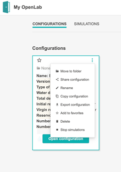
4.2 Configuration actions
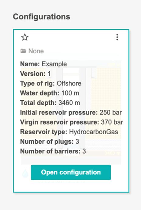
After a configuration has been created, it appears on the Home page. Moving the cursor over the configuration displays summary information and available actions. Select the three-dot menu to open the configuration action menu.
Typical actions include:
• move the configuration to a folder,
• rename the configuration,
• copy the configuration,
• delete the configuration,
• open or edit the configuration.
4.3 Edit a configuration
Open a configuration by selecting it from the Home page. The configuration editor shows the main input categories.

A recommended workflow is:
1. Fill in general well information and analysis scope.
2. Define the well architecture and annular segments.
3. Define the trajectory.
4. Define formations and mark reservoir/inflow zones.
5. Define reservoir properties and pressure evolution.
6. Define plugs and material properties.
7. Define barriers and select barrier elements.
8. Enable and parameterize failure modes.
9. Validate the setup and correct any error messages.
10. Run the simulation and review results.
The order matters. Later sections often depend on earlier inputs. For example, barrier elements are selected from plugs, annular segments, and impermeable formations that have already been defined.
5. General information and analysis scope
The General information section identifies the well and defines the analysis time window.
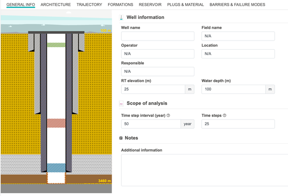
Recommended metadata includes:
• well name,
• field name,
• operator,
• location,
• responsible person,
• comments or notes describing assumptions,
• reference to the source of input data.
These fields may not all be required to run a simulation, but they are important for traceability. In practice, a simulation case is only useful if the assumptions behind it can be understood later.
5.1 Depth references
The depth reference information is important because well geometry, formation depths, casing depths, plug depths, and trajectory are interpreted relative to the selected reference. The guide and legacy manual use measured depth (MD) and true vertical depth (TVD). Rotary table or rotary kelly bushing elevation may be used as a depth reference, depending on the implementation.
For offshore wells, define the water depth when required. This is used for the schematic and may also affect conversion of rates to seabed or standard conditions in result views.
5.2 Scope of analysis
The analysis scope defines how far into the future the simulation should evaluate the barrier system.
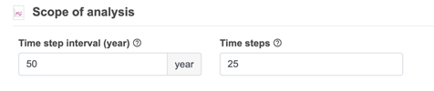
The current guide uses a standard example of 50 years per time step and 25 time steps, corresponding to a total analysis period of 1,250 years. These values can be changed. Use an analysis period that is meaningful for the question being asked. A shorter period may be suitable for comparing designs over an operationally relevant time frame. A longer period may be useful for understanding long-term leakage potential.
The selected time step affects pressure evolution, stress evolution, result plots, and the time points at which leakage is reported. More time steps provide a finer time resolution, but may increase simulation time.
6. Well architecture
The Architecture section defines the casing program, annular segments, and open-hole section.
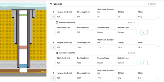
For each casing, define:
|
Input |
Meaning |
Notes |
|
Hanger or suspension depth |
Start depth of the casing |
Measured depth |
|
Shoe depth |
End depth of the casing |
Measured depth |
|
Length |
Distance between start and end depth |
Usually calculated automatically |
|
Open-hole diameter or hole size |
Diameter of the borehole for the
casing interval |
Used in geometry and schematic |
|
OD |
Casing outer diameter |
Required for interface geometry |
|
ID |
Casing inner diameter |
Required for internal geometry |
The legacy desktop guide emphasized that annular segments, rather than the casing object itself, are treated as well barrier elements. This distinction is important in the web version as well: a casing interval may be divided into different annular segments, and these segments may later be selected as barrier elements.
6.1 Annular segments
An annular segment describes a depth interval outside a casing or liner. A casing interval may be represented by one annular segment or split into several segments.


For each annular segment, define:
|
Input |
Meaning |
Notes |
|
Start
depth |
Start
of the annular interval |
Measured
depth |
|
End
depth |
End
of the annular interval |
Measured
depth |
|
Segment
type |
Default,
milled, or other type |
Mainly
descriptive unless linked to a model in the deployment |
|
Material
type |
Cement,
barite, Thermaset, Sandaband, other, or none |
Used
when the segment is part of a barrier |
Use several annular segments when only part of an annulus is cemented, when the annulus contains different materials, when a section has been milled, or when only a specific interval forms part of a well barrier.
Check that adjacent segments are continuous and do not overlap unless the intended model explicitly allows it. The first segment should normally start at the casing start depth, and the final segment should end at the casing shoe depth.
6.2 Open-hole section
If the well has an open-hole interval below the final casing, define the open-hole start depth, end depth, length, and diameter. The open-hole interval may affect formation exposure, barrier definition, and interpretation of leakage pathways.
7. Trajectory
The Trajectory section defines the well path using pairs of measured depth (MD) and true vertical depth (TVD).
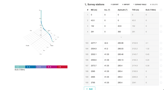
For a vertical well, at least two depth pairs are required: a start point and an end point. For deviated wells, add enough points to describe the trajectory with appropriate accuracy. The application calculates inclination and other trajectory-derived values from the MD/TVD pairs.
7.1 Import and export
Trajectory data may be entered manually or imported from a file. Export can be used to save a trajectory for reuse in similar configurations.
When editing trajectory rows, be careful with row order and depth consistency. The trajectory should extend at least to the deepest relevant formation top, plug, casing shoe, or open-hole depth used in the configuration.
7.2 Consistency checks
The trajectory must be consistent with the formation and casing inputs. If the trajectory ends above a formation or casing depth used elsewhere in the configuration, the application may not be able to calculate geometry-dependent values correctly.
Dogleg severity may be highlighted visually in the trajectory display. If the application reports a trajectory or dogleg error, review the MD/TVD pairs and check for unrealistic changes between adjacent points.
7.3 Legacy trajectory calculator
The legacy desktop version included a trajectory calculator that could estimate TVD from MD, or MD from TVD, once a valid trajectory had been defined. This concept remains useful even if the exact calculator is not visible in the web interface: use the trajectory to ensure that all depth-dependent inputs are interpreted consistently.
8. Formations
The Formations section defines the geological layers around the well.
A typical model includes several formations extending down to the reservoir. Each formation should be defined by a top measured depth and a rock type. The formation depth is often uncertain, so the top depth can be represented by a probability distribution.
8.1 Formation inputs
For each formation, define:
|
Input |
Meaning |
Notes |
|
Formation
name |
Unique
name used in the configuration |
Use
clear names such as “Shale caprock” or “Reservoir sand” |
|
Rock
type |
Geological
material |
Used
for interpretation and may affect stress-related calculations |
|
Top
depth MD |
Measured
depth to formation top |
Usually
represented as an uncertainty distribution |
|
Porosity |
Formation
porosity |
May
be optional depending on formation type and model |
|
Permeable |
Indicates
whether the formation can transmit fluid |
Permeable
formations are normally not selected as impermeable barrier elements |
|
Inflow
source / reservoir |
Marks
a permeable formation as a source of inflow |
At
least one reservoir/inflow source is normally required for simulation |
The legacy guide emphasized that the formation list does not need to represent a complete stratigraphic description. It should represent the formations needed for the leakage assessment, especially impermeable layers and any hydrocarbon- or CO2-bearing zones that may act as inflow sources.
8.2 Rock types
Available rock types may include:
• chalk,
• claystone,
• coal,
• limestone,
• marl,
• mudstone,
• permeable basalt,
• rock salt,
• sandstone,
• siltstone,
• shale,
• other formations.
Choose the rock type that best represents the formation. If the exact lithology is uncertain, document the assumption in the notes field.
8.3 Permeable and impermeable formations
Mark formations as permeable when they should allow flow or when they represent reservoir/inflow zones. Mark formations as impermeable when they may function as barrier elements. In later sections, only appropriate formations are normally available for selection as barrier elements.
8.4 Formation uncertainty
The exact top depth of a formation is often uncertain. Representing top depth as a distribution allows the Monte Carlo simulation to sample possible formation positions. This affects formation thickness and may affect contact between formations, plugs, and barrier elements.
9. Probability distributions
Many input parameters are uncertain. In OpenLab, uncertain inputs are indicated with a distribution icon.
Select the icon to open the distribution window.
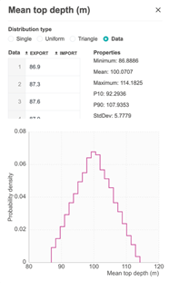
9.1 Common distribution types
The current web guide describes these distribution types:
|
Distribution |
Use case |
|
Single value |
Use when the value is known or when a
deterministic sensitivity case is needed |
|
Uniform |
Use when any value between a minimum and maximum
is considered equally likely |
|
Triangle |
Use when minimum, most likely, and maximum values
can be estimated |
|
Data |
Use when measured or sampled data should define
the distribution |
The legacy desktop guide also supported several advanced distributions, including normal, log-normal, exponential, Weibull, beta, gamma, chi-squared, Student’s t, F-distribution, discrete, generic data, and piecewise linear distributions. These are not necessarily visible in every web deployment. For most engineering input values, bounded distributions such as single value, uniform, triangle, or data-based distributions are preferred because they avoid unrealistic infinite tails.
9.2 Distribution selection guidance
Use a single value only when the value is known or when the purpose is to create a deterministic base case. Use a uniform distribution when only a credible lower and upper bound are known. Use a triangle distribution when expert judgement can provide a minimum, most likely value, and maximum. Use a data distribution when measured data are available and representative of the same physical property.
Avoid wide distributions unless they are justified. Very broad uncertainty ranges may dominate the result and make comparison between barrier designs difficult.
9.3 Documenting assumptions
For each important distribution, document:
• the data source,
• whether the value is measured, inferred, or based on expert judgement,
• the reason for the selected lower and upper bounds,
• whether the distribution is intended to be conservative, best estimate, or exploratory.
This is especially important for microannuli size, permeability, reservoir pressure, reservoir properties, and material mechanical properties.
10. Reservoirs and pressure evolution
The Reservoir section is used for formations that have been marked as reservoir or inflow source formations.
Reservoir inputs are important because leakage rates are strongly affected by pressure difference, fluid properties, and pressure evolution over time.
10.1 Reservoir type
The web guide describes reservoir types such as:
• hydrocarbon/gas,
• CO2.
Select the type that best represents the fluid source. The selected reservoir type may affect which fluid properties are required and how pressure and leakage are interpreted.
10.2 Pressure and temperature inputs
Typical pressure and temperature inputs include:
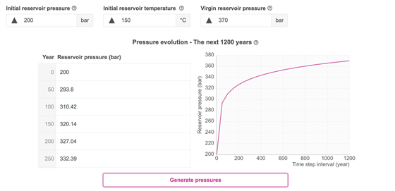
|
Input |
Meaning |
|
Initial reservoir
pressure |
Current reservoir
pressure at the start of the analysis |
|
Initial reservoir
temperature |
Reservoir temperature at
the start of the analysis |
|
Virgin reservoir
pressure |
Original undisturbed
reservoir pressure before depletion or injection history |
Pressure evolution may be entered manually or calculated automatically, depending on the implementation and selected options. In the legacy desktop version, if automatic pressure build-up was disabled, the user entered a pressure value for each defined time step. If automatic calculation was enabled, additional reservoir parameters such as initial volumes and productivity index were required.
10.3 Stress model and elastic properties
The calculator may include stress models to estimate the effect of far-field stress changes caused by long-term reservoir pressure changes.
Available stress model choices may include:
• Soltanzadeh,
• Geertsma,
• None.
The legacy manual recommended using the default stress model unless there is a clear reason to select another option. If None is selected, stress-related calculations and any time-to-failure model that depends on stress changes may not be available.
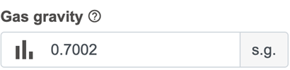
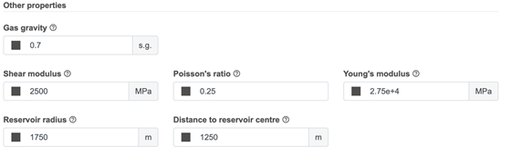
Typical stress and reservoir geometry inputs include:
|
Input |
Meaning |
|
Reservoir radius |
Assumed radius of
the reservoir volume used in the pressure/stress model |
|
Distance to
reservoir center |
Radial distance from
the well to the assumed reservoir center |
|
Shear modulus |
Elastic shear
stiffness of the formation |
|
Young’s modulus |
Relationship between
stress and strain in the formation |
|
Poisson’s ratio |
Ratio of transverse
strain to axial strain |
|
Gas gravity |
Reservoir gas
density relative to air |
10.4 Pressure evolution plot
The pressure evolution plot helps the user check whether the assumed pressure path is physically reasonable. Because leakage rate calculations are strongly dependent on pressure difference, pressure evolution should be reviewed before interpreting leakage results.
When the pressure evolution is manually specified, ensure that the final pressure is consistent with the intended long-term condition, such as re-pressurization toward virgin reservoir pressure. When pressure build-up is calculated automatically, check that the input volumes and productivity assumptions are reasonable.
11. Plugs, annular materials, and void materials
The Plugs and materials section defines permanent plugs and the properties of materials used in plugs and annular segments.

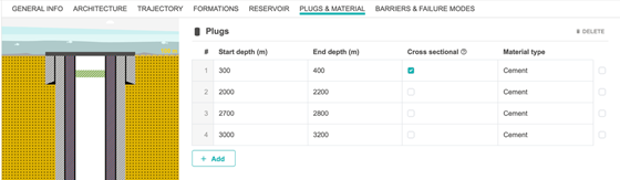
11.1 Plug geometry
For each plug, define:
|
Input |
Meaning |
Notes |
|
Start depth / plug top |
Top of the plug |
Measured depth |
|
End depth / plug bottom |
Bottom of the plug |
Measured depth |
|
Length |
Plug length |
Usually calculated from top and bottom |
|
Cross-sectional |
Indicates whether the plug extends across
the relevant cross-section |
May affect schematic and barrier
interpretation |
|
Material type |
Cement, barite, Sandaband, Thermaset, or
other |
Used to assign material properties |
All defined plugs are potential well barrier elements. A plug affects the simulation only after it is included in a barrier and relevant failure modes are enabled.
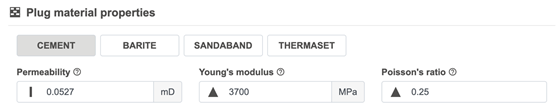
11.2 Material properties
Material properties are used by the failure-mode models. Typical inputs include:
|
Property |
Use |
|
Permeability |
Used for leakage through bulk
material |
|
Young’s modulus |
Used in stress and mechanical
response calculations |
|
Poisson’s ratio |
Used in stress and mechanical
response calculations |
The legacy desktop guide also described properties used for time-to-failure calculations:
|
Property |
Use |
|
Bond tensile strength |
Initial bond strength at the
material interface |
|
Stress caused by shrinkage |
Tensile stress induced during
hardening or hydration |
|
Bond strength reduction per year |
Assumed annual reduction in bond
strength over time |
These additional properties may be advanced or deployment-dependent in the current web version. When they are available, they should be specified only when the data source and assumptions are clear. Time-to-failure predictions are sensitive to degradation assumptions.
11.3 Default material values
Default values may be available for some materials. Treat them as examples or fallback values, not as a recommendation. Project-specific material properties, laboratory measurements, or qualified expert estimates should be used whenever possible.
11.4 Void materials
Void material defines the fluid or medium present between plugs or above a plug.
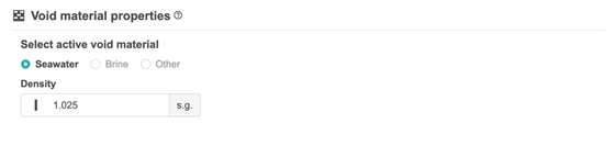
Options may include seawater, brine, or other fluids. The exact effect depends on the active models in the deployment. Even when void material has limited effect on the calculation, it should be documented to make the case description complete.
12. Barriers and well barrier elements
The Barriers section defines the permanent well barrier envelopes and the elements that make up each barrier.

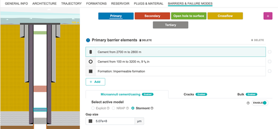
12.1 Barrier types
Common barrier types include:
• primary,
• secondary,
• open hole to surface,
• crossflow,
• tertiary.
The legacy desktop version also included categories such as common and none. Barrier types are primarily used for organization, visualization, and interpretation. The leakage calculation depends on the selected barrier elements and failure modes.
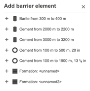
12.2 Well barrier elements
A well barrier is assembled from well barrier elements. Available elements are derived from earlier configuration sections and may include:
• plugs,
• annular segments,
• impermeable formations.

Every barrier should contain at least one barrier element. A simulation should not be considered meaningful until each barrier is properly defined.
A barrier element may be part of more than one barrier. The legacy manual noted that such elements were shown with special coloring in the schematic. In the web version, pay close attention to shared elements, because failure of a shared element may influence several barrier envelopes.
12.3 Barrier verification
The legacy desktop guide included a barrier verification section where the user could record verification methods based on NORSOK D-010. In the current web workflow, similar information may be stored in notes or dedicated verification fields if available.
Verification information is normally descriptive and does not automatically change the calculation. It is the user’s responsibility to ensure that verification results are reflected in the selected distributions and failure-mode assumptions. For example, good cement bond evidence may justify a lower microannuli size distribution, while uncertain verification may justify a broader distribution.
13. Failure modes
Failure modes define how a barrier element can leak.

The main failure modes are:
• microannuli,
• cracks,
• bulk leakage.
The available failure modes depend on the type of barrier element.
13.1 Failure modes for plugs

For plugs, typical failure modes are:
• microannuli at the plug/casing or cement/casing interface,
• cracks through the plug,
• bulk flow through the plug material.
13.2 Failure modes for casings and annular segments

For annular segments, typical failure modes include:
• microannuli at the cement/casing interface,
• microannuli at the cement/formation interface,
• cracks,
• bulk flow.
13.3 Failure modes for formations
For impermeable formation barrier elements, cracks may be the relevant failure mode. The available choices depend on the implementation and on how the formation has been defined.
13.4 Important interpretation of failure-mode checkboxes
The legacy manual makes an important modelling point: enabling a failure mode normally means that this failure mode is included in every Monte Carlo realization. The uncertainty is then expressed through the sampled defect size, permeability, aperture, or other input parameter. Disabling a failure mode means that it is excluded.
In other words, the checkbox is not necessarily a probability that the failure mode occurs. It is a modelling choice about whether that failure mechanism is active in the analysis. If multiple failure modes are enabled for the same barrier element, their effects are aggregated according to the model.
13.5 Failure mode overview

The failure-mode setup should be reviewed carefully before running a simulation. A common workflow is to begin with a simple case, enable one failure mode at a time, and then build up to the full combined case. This makes it easier to identify which assumptions control the results.
13.6 Microannuli models
Microannuli are a central part of the leakage calculation. They represent narrow flow paths along cement interfaces. The web guide describes three main microannuli size models.
Explicit model
The explicit model lets the user define microannuli size directly as a probability distribution. This is useful when the user has a direct estimate of gap size or wants to run a deterministic or controlled sensitivity case.
NRAP model
The NRAP model is based on the National Risk Assessment Partnership approach and uses probability classes for cement integrity. The user defines probabilities for quality classes such as good, medium, and bad integrity.
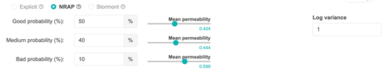
The probabilities across the selected classes should sum to 100%. The model then samples from the selected integrity class and converts the associated permeability representation to an equivalent microannuli size.
Stormont model
The Stormont model uses a relationship between effective wellbore permeability and microannulus hydraulic aperture. The user defines an effective wellbore permeability distribution, and the model converts this to a microannuli size distribution.
13.7 Microannuli grid and distribution
Microannuli may be represented as a grid of rows and columns. The grid is a simplified representation of vertical and lateral variability along the interface. The number of rows and columns affects both model resolution and calculation time.

Generate the grid or distribution to inspect the sampled microannuli sizes.
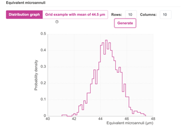
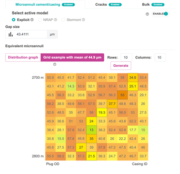
The legacy manual used a default 10 by 10 matrix and emphasized that the selected grid size may affect both results and computation time. Use a grid resolution that is consistent with the quality and resolution of the underlying data.
13.8 Cracks
Cracks are defects through a barrier element. Typical crack parameters include:
• aperture,
• orientation,
• width.
Each parameter may be uncertain and represented by a distribution. Crack inputs should be selected based on the physical scenario being modelled. A crack case may represent observed cracking, a conservative scenario, or a sensitivity case.
13.9 Bulk leakage
Bulk leakage represents flow through the barrier material itself. It is controlled primarily by material permeability and pressure difference. Bulk leakage may be important when the barrier material has relatively high permeability or when microannuli and cracks are excluded.
14. Simulation setup and validation
When the configuration is complete, start a simulation from the side menu.


The simulation dialog asks for a simulation name and the number of Monte Carlo iterations.
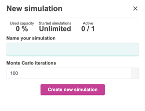
The current guide states that the number of iterations can be between 5 and 100,000, with 100 used as a default example. More iterations usually give smoother statistical results, but also increase calculation time.
14.1 Monte Carlo simulation
The calculator uses Monte Carlo simulation to propagate uncertainty in input parameters to uncertainty in leakage results. In each realization, values are sampled from the selected distributions. The model then calculates leakage rates for the active barriers, barrier elements, and failure modes. Repeating this process many times gives a distribution of possible outcomes.
Use a small number of iterations for quick debugging and validation. Use a larger number when comparing designs or reporting results.
14.2 Simulation time settings
The simulation time settings are linked to the analysis scope. The legacy guide described two key parameters: number of time steps and time-step interval in years. Their product defines the maximum analysis time.
For example:
|
Number of time steps |
Time-step interval |
Total analysis time |
|
25 |
50 years |
1,250 years |
|
50 |
20 years |
1,000 years |
|
100 |
10 years |
1,000 years |
Choose a time resolution that captures the expected pressure and stress evolution. Very coarse time steps may miss important changes. Very fine time steps may increase computation time without improving the decision.
14.3 Validation and error messages
Before or during simulation, the application validates the configuration. Validation may identify missing values, impossible geometry, inconsistent depth intervals, invalid distributions, missing reservoirs, undefined barriers, or failure modes without required parameters.
Use validation messages as a checklist. Do not ignore warnings unless you understand why they do not affect the specific analysis.
15. Results and interpretation
After the simulation has been created, OpenLab opens the result panel.
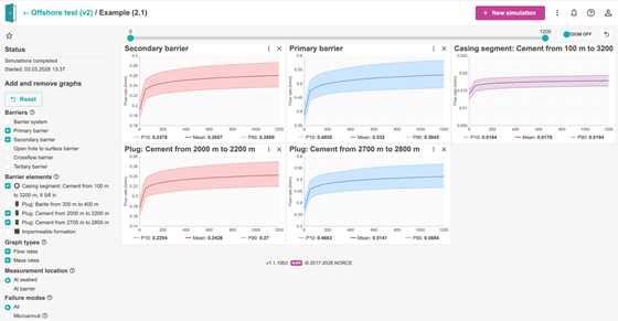
The result panel is interactive. Users can select which graphs to show, move graph panels, resize them, and inspect different result categories.
15.1 Graph selection
The graph selection panel allows the user to choose what results to display.
Available choices may include:
|
Category |
Typical options |
|
Barrier selection |
All barriers or selected barriers |
|
Barrier element selection |
Casings, plugs, or impermeable formations |
|
Graph type |
Flow rate or mass rate |
|
Measurement location |
At seabed or at barrier |
|
Failure mode |
All, microannuli, cracks, bulk |
|
Microannuli interface |
Plug/casing, cement/casing, cement/formation |
The exact list depends on the configuration and deployment.
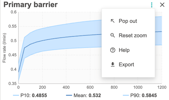
15.2 Graph panel menu
Each graph has a menu in the upper-right corner.

Typical graph menu functions may include opening, copying, exporting, resizing, or changing display settings. In the legacy desktop version, plots also supported context menus for showing percentiles, mean values, cumulative distribution functions, copying plot images, exporting data, changing units, and opening plots in separate windows. Similar functionality may be available in the web result panel through graph menus or export features.
15.3 Leakage rate interpretation
Leakage rate is the primary result for many analyses. The legacy manual distinguished between system-level, barrier-level, and barrier-element-level leakage rates:
• System leakage rate represents the leakage through the overall barrier system.
• Barrier leakage rate represents the leakage through a selected well barrier.
• Barrier element leakage rate represents leakage through an individual element such as a plug, annular segment, or impermeable formation.
In a series-connected barrier interpretation, the lowest barrier leakage rate can act as a bottleneck for the system. In a parallel or aggregated interpretation within a barrier, contributions from barrier elements and failure modes may be summed according to the model.
When interpreting leakage rate results, check:
• whether rates are reported at the barrier or converted to seabed/standard conditions,
• whether the plotted rate is flow rate or mass rate,
• whether all failure modes or only selected failure modes are included,
• which percentile, mean, or statistical value is being shown,
• whether the result represents a single time step or a time series.
15.4 Histograms and percentiles
Monte Carlo results should be interpreted as distributions, not single numbers. Useful statistics include:
|
Statistic |
Meaning |
|
Mean |
Average result across all realizations |
|
P10 |
10th percentile; 10% of realizations are below this
value |
|
P50 |
Median result |
|
P90 |
90th percentile; 90% of realizations are below
this value |
|
Minimum/maximum |
Range of sampled outcomes; may be sensitive to
outliers |
When reporting results, specify which statistic is used. A P90 leakage rate represents a more conservative value than the mean or P50.
15.5 Cumulative leakage volume
Some result views may show cumulative leakage volume over time. This is calculated from leakage rates over the simulated time interval. Interpret cumulative volume with care: it assumes no intervention, no change in barrier condition beyond the model assumptions, and no external operational changes during the analysis period.
15.6 Importance analysis
The legacy desktop version included importance analysis results showing which barrier or failure mode most often controlled the system result. This concept is valuable in the web version as well. Use importance-style results to answer:
• Which barrier is most often the bottleneck?
• Which failure mode contributes most to leakage?
• Which barrier element is most important for risk reduction?
These results can guide design improvements and data acquisition. For example, if microannuli at the cement/formation interface dominate, improved cement placement, verification, or narrower microannuli assumptions may be more important than changing bulk material permeability.
15.7 Sensitivity analysis
The legacy manual described sensitivity analysis for plug length, plug location, and plug material. Even if the current web deployment implements sensitivity in a different way, the same interpretation applies.
A useful sensitivity workflow is:
1. Define a base case.
2. Vary one parameter or design choice at a time.
3. Compare leakage rate and uncertainty range.
4. Identify changes that produce meaningful reduction in leakage.
5. Check whether the change is physically and operationally realistic.
Common sensitivities include plug length, plug depth, material permeability, microannuli size distribution, crack aperture, reservoir pressure, and stress model assumptions.
15.8 Pressure evolution results
Pressure evolution results show how reservoir pressure changes during the analysis period. Since leakage depends strongly on pressure difference, pressure plots should be reviewed before interpreting leakage trends.
If leakage increases with time, check whether this is caused by reservoir pressure build-up, stress-induced microannuli changes, degradation assumptions, or a combination of effects.
15.9 Stress and microannuli results
Advanced result views may show stress changes and microannuli evolution. These are useful for understanding whether far-field stress changes or material shrinkage may increase interface openings over time.
When stress results are available, check:
• which stress model was used,
• whether the required elastic properties are well constrained,
• whether microannuli growth is dominated by the initial microannuli model or by stress-induced changes,
• whether the selected material mechanical properties are realistic.
15.10 Time-to-failure results
The legacy desktop version included time-to-failure calculations based on a Bayesian approach using NCS P&A well data and stress/degradation assumptions. These results were separate from leakage-rate calculations, although leakage had to be positive for failure criteria to be reached.
If time-to-failure outputs are available in your OpenLab deployment, interpret them as model-based indicators rather than direct predictions. They are sensitive to:
• bond strength,
• shrinkage stress,
• annual bond strength reduction,
• far-field stress model,
• reservoir pressure evolution,
• assumed prior failure data.
If no stress model is selected, legacy time-to-failure calculations may not be performed because the failure criterion depends on stress changes.
15.11 Comparative analysis
The legacy desktop version included a comparative analysis view for comparing a base case and an alternate case. In the web version, similar comparisons can be made by copying configurations, changing one design feature, and running a new simulation.
When comparing two configurations, keep all non-tested inputs unchanged. Otherwise, differences in results may be caused by several changes at once and become difficult to interpret.
16. Other application features
Additional features are available from icons in the simulation window.

16.1 More menu
The More menu includes functions for unit system, sharing, download, and import.
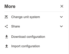
Change unit system
The application can display values in different unit systems.
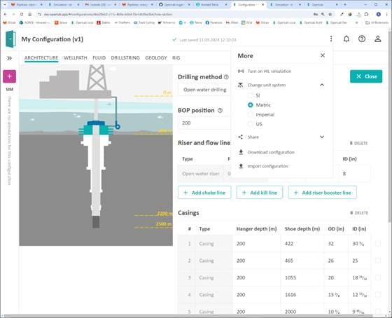
Typical options include:
• SI or base units,
• metric units,
• imperial (UK),
• US customary units.
The legacy desktop version also included industry and oilfield unit sets and custom display precision. In any version, always check unit labels before entering or interpreting values.
Share button
The share function may copy a page link to the clipboard or open a standard email application with a link to the simulation. Configurations and simulations have unique identifiers in the browser URL. These links should be shared only with users who have the required access rights and authorization.
Download configuration
After or before simulation, the configuration can be downloaded as a structured file such as JSON. Store the file safely and remember that it may contain readable well and project data.
Import configuration
An existing configuration can be imported from a file. After import, review the configuration carefully before running a simulation. Unit systems, available features, and validation rules may differ between versions.
16.2 Error messages and Jill-Bit
If the configuration contains errors or warnings, an error icon or notification may appear. The application includes the Jill-Bit assistant to help identify the source of the error and suggest how to correct it.
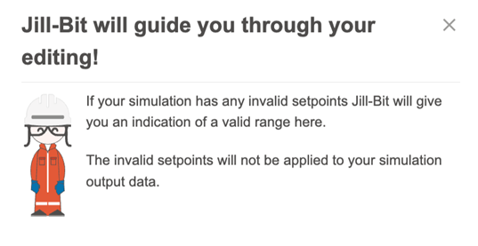
Use error messages to correct missing input, inconsistent geometry, invalid distributions, or incomplete barrier definitions.
16.3 Help menu
The help menu provides access to user guidance and support resources.
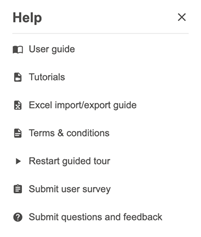
Functions may include:
• opening the user guide,
• viewing tutorials,
• opening the Excel import/export guide,
• viewing terms and conditions,
• restarting the guided tour,
• submitting a user survey,
• submitting questions or feedback.
16.4 User menu
The user menu provides access to profile, license, and settings information.

Use this menu to check account-related information and user-specific settings.
17. Good modelling practice
17.1 Start simple
Begin with a simple configuration and one or two active failure modes. Confirm that the model behaves as expected before adding more complexity.
17.2 Keep assumptions visible
Use notes fields to document the source of key inputs. This is especially important for uncertain parameters such as microannuli size, reservoir pressure, permeability, crack aperture, formation depth, and material properties.
17.3 Use templates carefully
Templates are useful starting points, but they are not a substitute for case-specific validation. Replace template values with project-specific values whenever possible.
17.4 Validate geometry
Check that casing depths, plug depths, formation depths, annular segments, and trajectory are mutually consistent. Geometry errors can be difficult to diagnose after simulation.
17.5 Interpret uncertainty, not only averages
Monte Carlo simulations produce a distribution of outcomes. When comparing cases, compare P10/P50/P90 or other agreed percentiles, not only mean values.
17.6 Be explicit about what is excluded
A failure mode that is disabled is not included in the simulation. Document why it is excluded. A disabled failure mode does not mean that the failure mechanism is physically impossible; it means that it is outside the selected model case.
17.7 Compare like with like
When comparing alternative P&A designs, keep all assumptions identical except for the design change being tested. This makes the interpretation clearer and more defensible.
Appendix A. Legacy and advanced features
This appendix summarizes useful technical information from the earlier desktop user manual. Some items may be available only in older versions or in specific OpenLab deployments.
A.1 Legacy system requirements
The old desktop version was a Windows application developed using Microsoft .NET 6.0. The current OpenLab version is web-based and does not require the old desktop installation. Users need a supported web browser and appropriate OpenLab access.
A.2 Legacy file handling
The old desktop version used XML project files and XML result files. The web version uses OpenLab-managed configurations and may export/import JSON configuration files. Both XML and JSON formats are readable text-based formats, so confidential project data must be handled carefully.
A.3 Acceptance criteria
The legacy desktop version included input sections for acceptance criteria. These criteria were mainly used for visualization and color coding, not for changing simulation physics.
Leakage-rate acceptance criteria
The user could define lower and upper acceptable leakage-rate limits. In current workflows, acceptance criteria should be derived from relevant regulations, company policy, project requirements, or study-specific decision criteria.
Log-quality acceptance criteria
The legacy manual described log-quality categories for cement and other materials using high, medium, and low bond quality categories. These categories could be applied to VDL/CBL, acoustic impedance, and flexural attenuation logs. The values should be treated as case-specific interpretation limits, not universal acceptance limits.
A.4 Log-based microannuli models
The legacy desktop version included models that converted cement bond log images to microannuli size distributions. These models required an image of the log, definition of the log type and color scale, and a mapping function from log value to microannuli size.
Supported legacy log types included:
• gamma ray,
• neutron,
• VDL/CBL,
• acoustic impedance,
• flexural attenuation,
• resistivity,
• microannuli interpretation,
• sonic,
• user-defined.
Supported color interpretations included brightness, RGB, BGR, and custom color scales. The user could define minimum, midpoint, and maximum colors and exclude non-log colors. The model then interpreted the image into a matrix of log values and mapped these values to microannuli sizes.
A multiple-log model allowed several logs to be combined using probabilistic weights. This could be used when different logs described the same interval under different conditions or with different uncertainty levels.
These log-based workflows are powerful but sensitive to image quality, color scale selection, log depth alignment, and the mapping function. Use them only when the underlying log interpretation is well documented.
A.5 Failure data and Bayesian time-to-failure model
The legacy desktop version included a static data set based on permanently plugged wells on the Norwegian Continental Shelf. The manual stated that the extraction was from the Norwegian Petroleum Directorate fact pages and that the most recent extraction in that version was performed on 25 May 2021. The data were used as part of a Bayesian time-to-failure calculation.
The legacy manual also stated that no registered leaks were found in that data extraction, and the user could modify the assumed number of failures. Because this is version-specific and based on a static historical extraction, do not treat it as current failure statistics unless the data source has been updated and verified in the current deployment.
A.6 Design-related and long-term failure placeholders
The legacy desktop manual described input sections for design-related failures and long-term effects as placeholders for future models and recommended not setting those parameters unless there was a clear reason. The same general caution applies to any advanced input that is not part of the validated workflow in the current deployment.
Appendix B. Terminology
|
Term |
Meaning |
|
Barrier |
A well barrier envelope, such
as a primary or secondary barrier |
|
Barrier element |
A physical element that
contributes to a barrier, such as a plug, annular segment, or impermeable
formation |
|
Bulk leakage |
Flow through the barrier
material itself |
|
Configuration |
The full OpenLab case
definition used for a simulation |
|
Crack |
A discrete defect through a
barrier element |
|
Distribution |
A probability model used to
represent uncertain input values |
|
MD |
Measured depth along the
wellbore |
|
Microannulus |
A narrow flow path along an
interface, commonly cement/casing or cement/formation |
|
Monte Carlo simulation |
Repeated sampling of
uncertain inputs to estimate a distribution of possible results |
|
P10/P50/P90 |
Percentiles used to describe
uncertainty in simulation results |
|
Reservoir/inflow source |
Formation that can provide
fluid or gas driving leakage |
|
TVD |
True vertical depth |
|
Void material |
Fluid or medium present
between or above plugs |
Document status
This consolidated guide is intended for editorial review and technical checking before publication in Ghost or distribution as a Word document. Screenshots are from the current OpenLab web guide. Legacy modelling explanations have been adapted to the current web workflow and should be checked against the deployed OpenLab feature set before final release.
Dan Sui Associate Professor at UiS
Department of Energy and Petroleum Engineering

Mats Hermansen
SVP Sales, Exebenus


